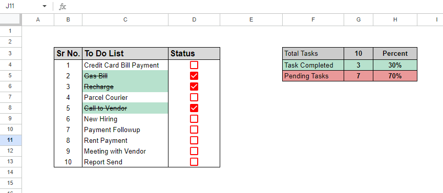
Creating a checklist in Google Sheets is a fantastic way to organize your tasks, projects, or even personal to-dos. In Google Sheets we can create checklist or to-do list easily to manage and share with other. Here below is a image for simple checklist in Google Sheets image.

Step-by-Step Guide to Creating a Checklist in Google Sheets
Step 1: Create New Google Sheets File
First Create New Google Sheets file and rename your Sheet. If you don’t know how to create new Google Sheets then you can you can read Google Sheets Basic Tutorial.
Step 2: Set Up Your Range
Decide what columns you need for your checklist. Typically, you’ll want at least three columns: one for the checkbox and another for the task description and another for serial number of tasks. You can add more columns as your preference. In this tutorial using B column to D column. First row add Headers in Google Sheets. In this tutorial adding Headers to B3:D3 as Sr No., To Do List and Status. You can change your range in your Google Sheets as your preference.
- Column B: In this column you can add serial number.
- Column C: This column will be task descriptions.
- Column D: This column will be checkbox column where you can tick on them if task is completed.
Step 3: Enter your Tasks
In C column, start entering the tasks that you want to include in your checklist. For example.
- Credit card bill payment in C4.
- Gas bill in C5.
- Recharge Wi-Fi in C6 etc.
Step 4: Use formula to automatic serial number
Use below formula in B4 cell so that serial number automatically insert when new task added.
=IF(C4=“”,“”,SEQUENCE(COUNTA(C4:C),1,1))
in above formula C4:C means Task starting Cell to whole task column. You can also convert this formula to Array formula.
Step 5: Insert Checkboxes
To insert check boxes in Google Sheets first of all select the range where you want to insert checkboxes. For example D4:D13 and go the Insert Menu in the top of Google Sheets then click on Checkbox then you can see there are Checkboxes. You can also set colors to Checkboxes by clicking on Text color option. In below image applied red color to checkboxes.
Step 6: Apply Conditional Formatting
To apply conditional formatting follow these steps in Google Sheets:
- Select Tasks columns for example C4:C13.
- Go to Format menu and click on Conditional formatting.
- Under “Format cells if”, click on dropdown and choose Custom formula and enter the formula
=D4=TRUE
if you want use conditional formatting B4:C13 (Serial Number and Tasks Column) then select this range and use formula: =$D4=TRUE.
- Choose Formatting style such as Fill color light Green and strikethrough. You can choose more formatting style as per your preference.
- Click on Done.
Step 7: Tasks Progress Dashboard (Optional)
To make Tasks Progress Dashboard Type headers in in F3:F5 as Total Tasks, Task Completed and Pending Tasks. You can change range as per your preference.
Write formula in G3. =COUNTA(C4:C13)
in G4. =COUNTIFS(D4:D13,TRUE)
and in G5. =COUNTIFS(D4:D13,FALSE)
in H3 Type Percent or any suitable header name.
and write formula in H4 =G4/G3 and in H5 =G5/G3.
Now select G4 and G5 and convert number to % (percentage) format by clicking on Format as percent or press keyboard shortcut key Ctrl + Shift + 5.
Step 8: Share your Checklist (Optional)
If you need to collaborate with others then you can share your Google Sheets checklist. To share Click the “Share” button in the top-right corner of Sheets, enter the email addresses of the people you want to share with, and set their permission level Viewer, Commenter, or Editor).
Conclusion
Creating a checklist in Google Sheets is simple yet powerful way to stay organized. With just a few clicks, you can set up a dynamic checklist that helps you track tasks, improve productivity, and collaborate with others easily. Whether you’re managing personal tasks or working on a team project, Google Sheets offers the flexibility and features you need to create an effective checklist.